
Objective#
The objective of this project is to be able to predict how highly rated a coffee would be on CoffeeReview.com based purely on information about the coffee such as:
- Origin
- Roaster and roasting style
- Price
- Flavour profile
I will use this dataset from Kaggle which contains ratings for ~1900 coffees.
Data processing#
I will begin by loading in the data into a pd.DataFrame and also renaming the columns to more clearly distinguish between the country of origin and roaster country.
import pandas as pd

df = pd.read_csv("./data/simplified_coffee.csv")
for col in ["name", "roaster", "roast", "loc_country", "origin", "review"]:
    df[col] = df[col].astype("string")

df["review_date"] = pd.to_datetime(df["review_date"])
df = df.rename(columns={"loc_country": "roaster_country", "100g_$": "price_per_100g", "origin": "country_of_origin"})
df.head()| name | roaster | roast | roaster_country | country_of_origin | price_per_100g | rating | review_date | review |
|---|---|---|---|---|---|---|---|---|
| Ethiopia Shakiso Mormora | Revel Coffee | Medium-Light | United States | Ethiopia | 4.70 | 92 | 2017-11-01 | Crisply sweet, cocoa-toned. Lemon blossom, roa… |
| Ethiopia Suke Quto | Roast House | Medium-Light | United States | Ethiopia | 4.19 | 92 | 2017-11-01 | Delicate, sweetly spice-toned. Pink peppercorn… |
| Ethiopia Gedeb Halo Beriti | Big Creek Coffee Roasters | Medium | United States | Ethiopia | 4.85 | 94 | 2017-11-01 | Deeply sweet, subtly pungent. Honey, pear, tan… |
| Ethiopia Kayon Mountain | Red Rooster Coffee Roaster | Light | United States | Ethiopia | 5.14 | 93 | 2017-11-01 | Delicate, richly and sweetly tart. Dried hibis… |
| Ethiopia Gelgelu Natural Organic | Willoughby’s Coffee & Tea | Medium-Light | United States | Ethiopia | 3.97 | 93 | 2017-11-01 | High-toned, floral. Dried apricot, magnolia, a… |
We should check for any NaNs:
df.isna().sum()| name | 0 |
|---|---|
| roaster | 0 |
| roast | 12 |
| roaster_country | 0 |
| country_of_origin | 0 |
| price_per_100g | 0 |
| rating | 0 |
| review_date | 0 |
| review | 0 |
The roast column is the only one containing NaNs. Since there are only 12 missing values, we could just remove these rows. However, since most coffees have the same roasting style (as will see later), let us fill with the modal value.
df["roast"] = df["roast"].fillna(df["roast"].mode().iloc[0])Let’s fix a typo in the roaster country for one coffee.
df["roaster_country"] = df["roaster_country"].str.replace("New Taiwan", "Taiwan")Some roasters such as “El Gran Cafe” are duplicated since they entered with slightly different spellings in different rows (eg sometimes with the accented é and sometimes with a plain e). I will rename the roasters consistently by replacing these characters:
replace = {"’s": "'s", "é": "e", "’": "'"}
for k, v in replace.items():
    df["roaster"] = df["roaster"].str.replace(k, v)
We should also verify that the information about each roaster (in this case only country) is consistent across all coffees from the same roaster.
def _assert_identical_values(df: pd.DataFrame) -> pd.Series:
    assert (df.iloc[1:, :] == df.iloc[0, :]).all().all()
    return df.iloc[0, :]
Region of origin#
Most coffees come from certain regions of the world, and the coffees from each region tend to be similar in flavour profile (eg African coffees are typically more acidic and South American coffees more nutty.) Therefore it may be useful to categorise the countries by region.
The mapping from regions to countries has been manually compiled and stored in regions.json. We need to load this JSON file, invert the mapping so that it goes from country to region, and then engineer a new column for the region.
with open("./data/regions.json", "r") as f:
    REGIONS = json.load(f)

regions = {}
for r, countries in REGIONS.items():
    for c in countries:
        regions[c] = r

df["region_of_origin"] = df["country_of_origin"].map(regions).fillna("Other")
Flavour notes#
As it stands, we cannot glean any information from the review column as it is unstructured. Let’s begin by analysing the keywords present in the reviews using the WorldCloud package:
from wordcloud import WordCloud, STOPWORDS

COFFEE_WORDS = {"cup", "notes", "finish", "aroma", "hint", "undertones", "mouthfeel", "structure", "toned"}

word_cloud = WordCloud(collocations=False, width = 1000, height = 500, background_color='white', stopwords=set(STOPWORDS) | COFFEE_WORDS).generate(
    " ".join(df["review"])
)
plt.imshow(word_cloud)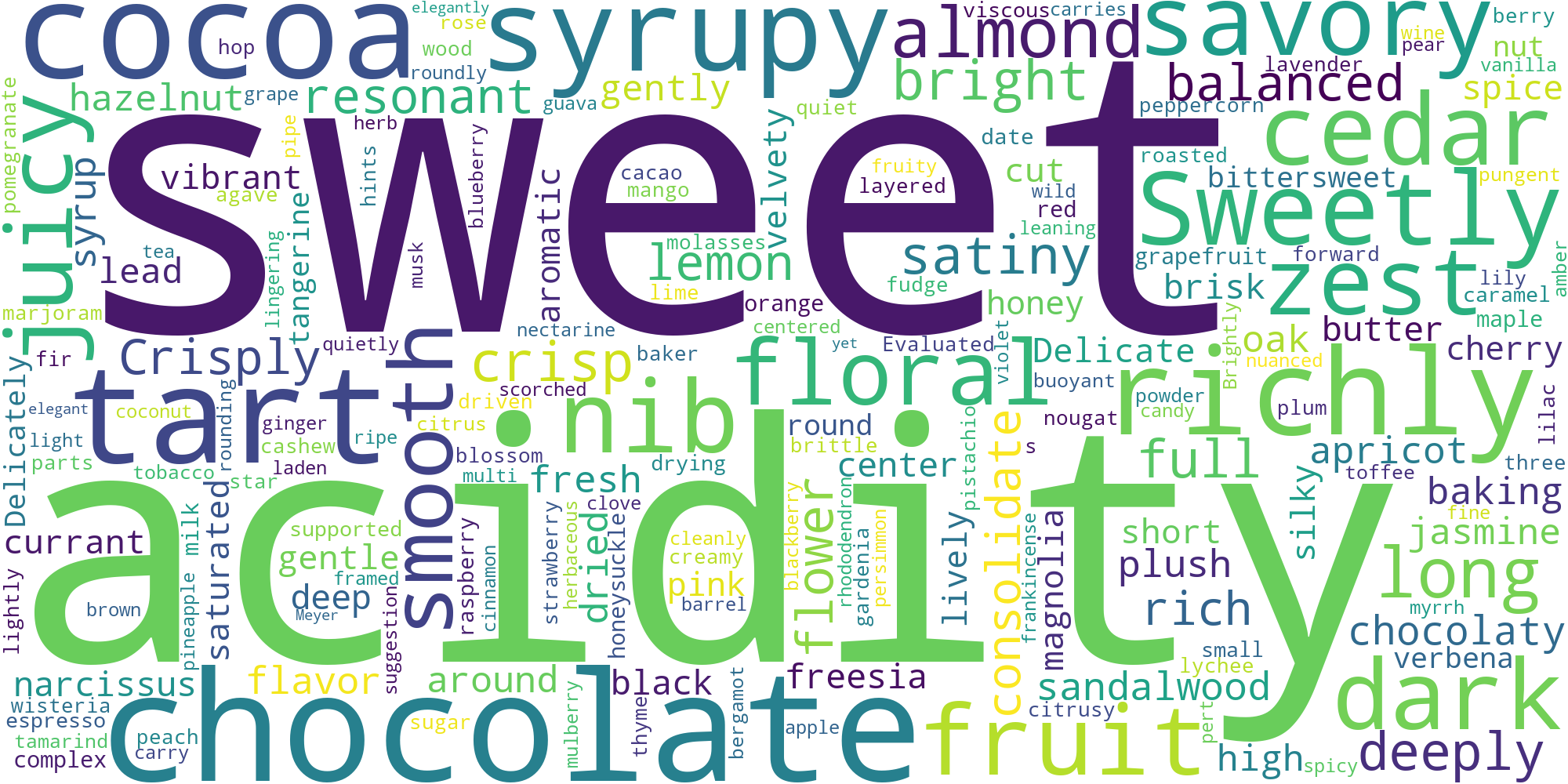
Note that we have had to remove common coffee-related nouns, which is assumed provide no information about the particular coffee. We can see that the most common words relate to the flavour of the coffee such as “acidity” or “chocolate”. This suggests that we can extract some features for the different flavours in the coffee.
Using this insight and the coffee flavour wheel, we can manually define some flavours and corresponding keywords which are stored in flavours.json.
with open("./data/flavours.json", "r") as f:
    FLAVOURS = json.load(f)
We can now engineer boolean features for each flavour.
def rating_contains_words(review: str, keywords: list[str]) -> bool:
    words = extract_words(review)
    for w in keywords:
        if w in words:
            return True
    return False


for flavour, keywords in FLAVOURS.items():
    df[flavour] = df["review"].apply(rating_contains_words, args=(keywords,))
It is also interesting to check how many flavours the different coffees have. If we have done a good job at defining the flavour keywords, we would expect that mode coffees would:
- Have at least some flavours since this is a key component of any review
- Not have an excessive number of flavours, as this would indicate we have chosen too “common” keywords
df[list(FLAVOURS.keys())].sum(axis=1).hist()Indeed, this appears to be the case. All coffees have at least 2 flavours, and in fact most coffees have ~6 flavours.
Distributions of each feature#
We will begin by exploring the distribution of each feature in the dataset.
Rating#
We can see that the ratings appear to be approximately normally distributed. However, the median rating is surprisingly high at ~94% and the standard deviation is low, so that the effect rating range ranges roughly from 85-100.
df["rating"].hist()Price#
The distribution for the price of the coffee is shown below.
df["price_per_100g"].hist()There is a very long tail, due to a few very expensive coffees. This suggests that there may be a benefit in applying the log transformation when we come to fit the model.
Roasting style#
The vast majority of the coffees have the medium-light roast type. This large bias in the dataset may make it challenging for a model to detect any impact of roasting style on coffee rating.
df["roast"].hist()Roaster country#
If we look at the value counts, we see that most of the coffees are from US roasters.
df["roaster_country"].value_counts()| roaster_country | |
|---|---|
| United States | 774 |
| Taiwan | 339 |
| Hawai’i | 77 |
| Guatemala | 24 |
| Hong Kong | 9 |
| Japan | 8 |
| England | 7 |
| Canada | 5 |
| Australia | 1 |
| China | 1 |
| Kenya | 1 |
If we look at the distribution of pricing for the most common countries, we see that the distribution is quite different in each country. In particular, the distribution of coffees from US roasters has a much more pronounced peak at the lower price level. This likely indicates that there is some bias in the dataset. Given that CoffeeReview is based in the US, they have reviewed a disproportionate number of more affordable coffees from US roasters.
countries = ["United States", "Taiwan", "Guatemala"]
df[df["roaster_country"].apply(lambda c: c in countries)].histogram("price_per_100g",by="roaster_country")Origin#
Country of origin#
We will first examine the different countries of origin in the dataset:
df["region_of_origin"].hist()As expected, most of the coffees come from the largest coffee producing countries in the world, almost a third are from Ethiopia alone.
Region of origin#
We also plot the regions of origin:
df["region_of_origin"].hist()Almost all examples are from one of the following regions which are the major coffee producing regions of the world:
- East Africa such as Ethiopia or Kenya
- Central or South America such as Colombia or Guatemala
There are also a lot of coffees from Hawaii, which is likely again because the data is from a US-based website.
Flavour#
In order to examine the popularity of the different flavours, we can plot the histogram:
df[list(FLAVOURS.keys())].sum().divide(df.shape[0]).sort_values(ascending=False).plot.bar()We can see that the most common flavours are:
- Caramelly
- Acidic
- Fruity
- Chocolate
Intuitively, this makes sense as these are the sorts of flavours seen mentioned on packets of coffee.
Influence of features on rating#
We can now move onto trying to identify any influence of the different features on the rating of the coffee.
Price#
To visualise the influence of price on the rating, we can simply produce a scatter plot:
df.plot.scatter(x="price_per_100g", y="rating")There appears to be some positive correlation between the two variables, although there is a fair amount of scatter so it is clear that there are other mechanisms at play here as well. This suggests that either:
- Price is genuinely an indicator of quality
- Price biases the reviewers
There is evidence of diminishing returns from increasing the price of the coffee, as the relationship between price and rating starts to flatten off.
Roaster#
If we look at the highest and lowest rated coffees, we see that they are dominated by certain roasters.
df.loc[df["rating"] > 96, ["name", "roaster"]].groupby("roaster").count()| roaster | count |
|---|---|
| Barrington Coffee Roasting | 1 |
| Bird Rock Coffee Roasters | 1 |
| Dragonfly Coffee Roasters | 1 |
| Hula Daddy Kona Coffee | 1 |
| JBC Coffee Roasters | 3 |
| Kakalove Cafe | 1 |
| Paradise Roasters | 2 |
df.loc[df["rating"] < 90, ["name", "roaster"]].groupby("roaster").count()| roaster | count |
|---|---|
| El Gran Cafe | 8 |
| Other | 4 |
To gain further insight, we can plot the average rating for the coffees with the most coffees:
roasters = df["roaster"].value_counts()
popular_roasters = sorted(roasters[roasters > 10].index)
df.groupby("roaster")["rating"].mean()[popular_roasters].plot.bar()
This is shown below, with the average rating across all coffees shown in black.
We can see that there is significant variation in the average rating for each roaster. For example, “El Gran Cafe” has a particularly low average rating around 3.0 below the average rating. This suggests that either:
- Certain roasters find the best/worst coffees or roast them particularly well
- The reviewers favour/dislike certainer roasters
Roasting style#
To assess if roasting style has an impact on the rating, we can plot the histogram grouping by the roasting style:
df.hist("rating", by="roast")It is clear that dark and medium-dark roasted coffees are often rated more poorly, since the tail has a significant skew to the left for these roasting styles. We can also see that the lighter roasted coffees have a much higher median rating, with medium roasted coffees somewhere in between.
We can plot the mean rating for each roasting style in the same way as for the roasters:
df.groupby("roast")["rating"].mean().plot.bar()As expected, the darker roasting styles have a much lower rating on average, which is because some of the darker roasted coffees are related particularly poorly. However, there is a much smaller difference between the light and medium-light roasting styles.
Origin#
Since there are many countries, we will analyse the influence of region of origin instead of country. We can plot the histogram of rating grouping by each region:
df.hist("rating", by="region_of_origin")We can see that the distribution for Central American coffees has a left-leaning tail, and the median is slightly lower than the other regions. However, we can glean more information by looking at the mean rating for each region of origin:
df.groupby("region_of_origin")["rating"].mean().plot.bar()This highlights that the East African coffees are more highly rated on average, and Central American are less highly rated. Therefore, there is evidence that the origin may have some influence on the rating of a coffee. However, the effect does not appear to be as strong as the roaster for example, since the difference between the highest and lowest average ratings is only around 0.5 compared to around 3.0 for the roaster.
Flavour#
To investigate the impact of flavour on rating, we can compute the average rating for coffees with and without each flavour, and compute the difference. If a flavour has a big impact on rating, we would expect to see a large difference.
rating_with_flavour = pd.Series({f: df.loc[df[f], "rating"].mean() for f in FLAVOURS})
rating_without_flavour = pd.Series({f: df.loc[~df[f], "rating"].mean() for f in FLAVOURS})
(rating_with_flavour-rating_without_flavour).hist("region_of_origin", by="roast")
We can see that for most flavours, the difference is quite small. However, it appears that fruitiness has a large positive influence and resinous a large negative influence on the rating.
Conclusions#
In this article, we has processed the coffee dataset and performed analysis to establish that:
- The dataset has a strong bias towards:
- Coffees from US roasters
- Coffees from East Africa or South America
- Medium-light roasted coffees
- We have detected which factors may be more likely to impact the rating:
- There is some definite correlation between price and rating
- Certain roasters have much higher and lower average ratings for their coffees, suggesting that this does impact the rating
- The roast style, origin and flavour profile all appear to have some impact on the rating, but it does not appear that the relationship is as strong as the roaster
In the next post, we will use the insight gained from this analysis to engineer features, and then training a predictive model.